Multi-ensemble based approach for Short-term Solar Radiation Forecasting
Introduction
This project consists of the development and implemetation of a modeling approach for solar radiation forecasting (although mostly as a “regression as forecasting”) from historical meteorological records using Machine Learning (ML) techniques. During the 12-month funding period, provided by FAPESP as a “Scientific Initiation” project, several activities such as literature review, data processing, model training and data analyses have been carried out resulting in a full ML pipeline. The data used in this project was collected by INMET, the National Meterology Institute in Brazil, consists of records of meteorological variables from which the models should learn; some of the treatments applied to the data, as well as other modeling decisions, are explained in futher details in following sections.
This project was originally inspired by this paper which showcases a similar approach for solar radiation prediction in Australia, where energy trading markets would benefit from intelligent systems capable of forecasting energy offer from photovoltaic solar predictions. Unfortunatelly, such markets are not available in Brazil as most of the electric energy comes from hydroelectric dams.
The implementation for this project was done in Python3 with common Data Science libraries such as Pandas, Scikit-Learn, Matplotlib, Numpy, GeoPandas and others.
Objective
The main objective of this project was to use Machine Learning techniques to predict solar radiation intensity, which can in turn be used to estimate the electric energy yeld from solar panel module. As this project was developed other sub-objectives were also divised to address this objective such as obtainig a data source, preprocessing the data and other operations related to training and testing of the methods. The sections to come highlight the work conducted in this project.
Data
Data Source
To achive the goal stablished in the section above, the dataset needed set of certain characteristics such as 1) contain the solar radiation variable, 2) hourly (or finer) record granularity and 3) contain measures of meteorological variables in multiple locations.
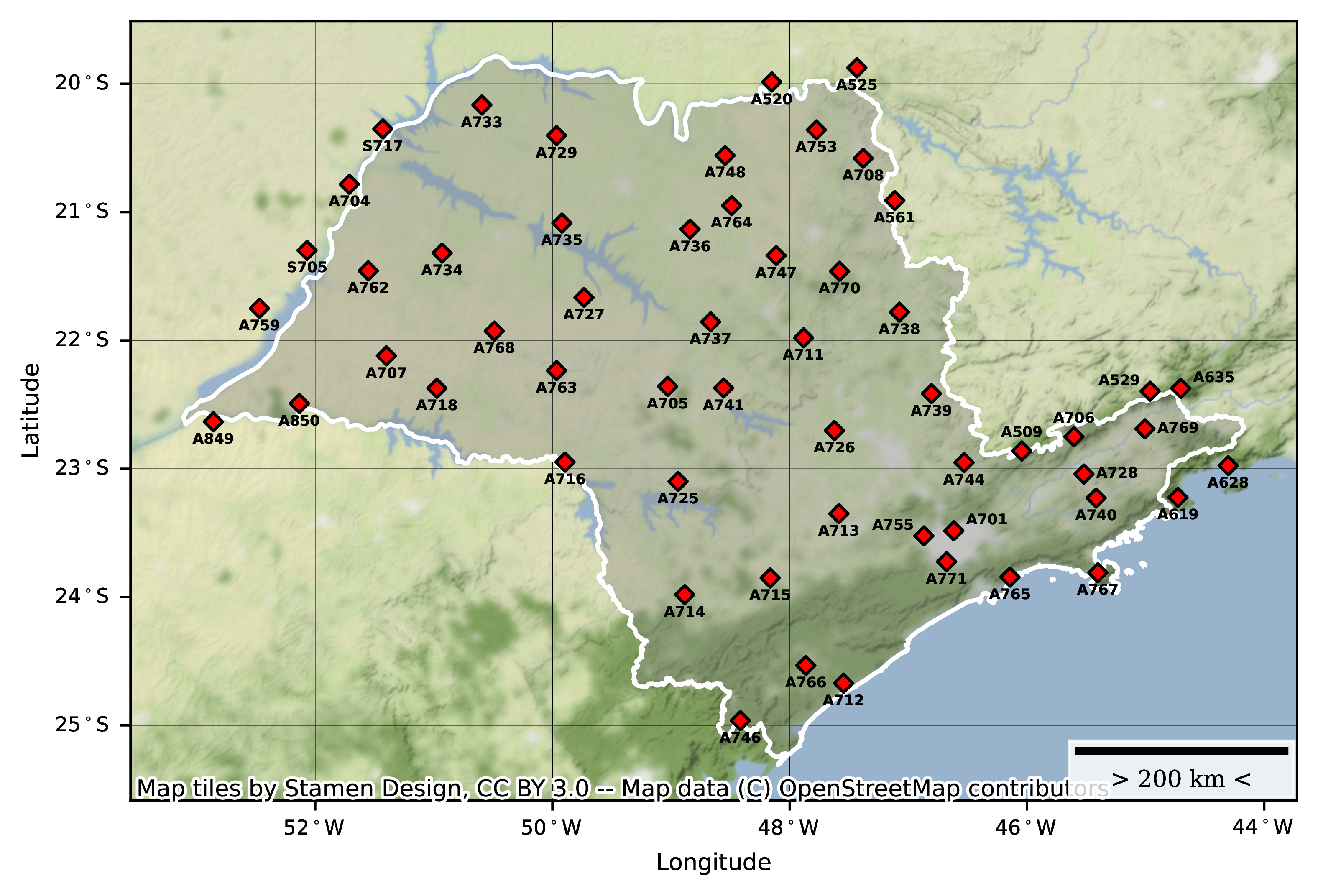
When this project was developed the only data source available with such attributes was provided by the Brazillian National Institute of Meteorology (INMET) through its website. The data, provided free of charge, is collected through several meteorological stations across the country on an hourly basis and transmitted to INMET for processing and storage. In order to limit the scope, only stations from the State of São Paulo, totallying 56 data collection sites, were seleted with records ranging from January 2001 to July 2021. The meteorological variables collected as well as the location of each meteorological station are shown below.
| Meteorologic variable | Unit |
|---|---|
| $B$ - Barometric pressure | hPa |
| $D$ - Dew point | °C |
| $H$ - Humidity | % |
| $P$ - Precipitatoin | mm |
| $T$ - Temperature | °C |
| $R$ - Global solar radiation | kJ/m² |
| $W_s$ - Wind speed | m/s |
| $W_d$ - Wind direction | ° |
Although the data provide by INMET was quite noisy in the hourly granularity, other applications depending on greater data granularities may benefit from the data provided by INMET as the network of data collecting stations is rather extense and well distributed across the country.
For more information access the Meteorological Station Map Explorer.
Preprocessing
Despite the availability, several issues had to be circumvented during data cleaning. Some of them worth mentioning are listed below:
Missing values: several meteorological station had major gaps due to availability problems. In some cases, all records from the station had to be discarted as the data would only introduce noise to the models during training. Despite not being documented, most of these issues with missing data must have originated from physical malfunction and/or damage in meteorological stations which remained unattended for several months.
Changes recording formatting: changes in formatting, introduced by migration of services or maybe restandardization of storage utilities, were also experienced. Examples of these changes include the way
NULLvalues were registered and date-time formatting changes.Change in stations’ geographical coordinates which affected distance relations. This issue had to be solved by manually searching the most recent coordinates for each station and retroactively overwriting them in historical records.
Some of the preprocessing operations carried out in the dataset to prepare this dataset envolved:
- PCA transforming $B$, $D$, $H$ and $T$ down to one component. These particular features had 3 measures associated to them in each hour: the maximum and minimum value within the hour as well as the instant measurement.
- Removing observations with spurious values, for example negative solar radiation or precipitation, temperatures inferior to 10°C as these are extremely rare in the area of study, solar radiation greater than 8000 kJ/m², etc.
- Applying a data imputation technique as an attempt to reconstruct at least part of the data lost due to data quality problems (see section Data Imputation).
- Filtering the stations based on number of observations as only stations with relevant amount of years of observation were necessary to build the train and test sets. For this filtering, only stations with 7 years worth of valid observations were considered.
- Reformatting datetime columns in order standardize the observations and properly adjust the daylight saving time across the years (some of the years in records had an extra daylight saving hour which had to be accounted for; others didn’t, which caused inconsistencies).
- Adjusting of target variable, which envolved first filtering the observations to select only a fixed window for the observations, i.e. only hourly observations between 7:00 and 18:00 (local time) were selected. After the operations of normalizing daylight saving time and selecting the proper time window, the solar radiation could safely be shifted in one hour ahead to get the associated value for the next hour.
- Data normalization using the Robust Scaler.
- Applying temporal holdout split to obtain the train and test sets. Out of the Jan/2001 to Jun/2021 period available when this project was developed, 2001-2018 (inclusve) was selected for training and the remaining data (2019-2021) for testing. After the split, the observations in the training set were shuffled.
Data Imputation
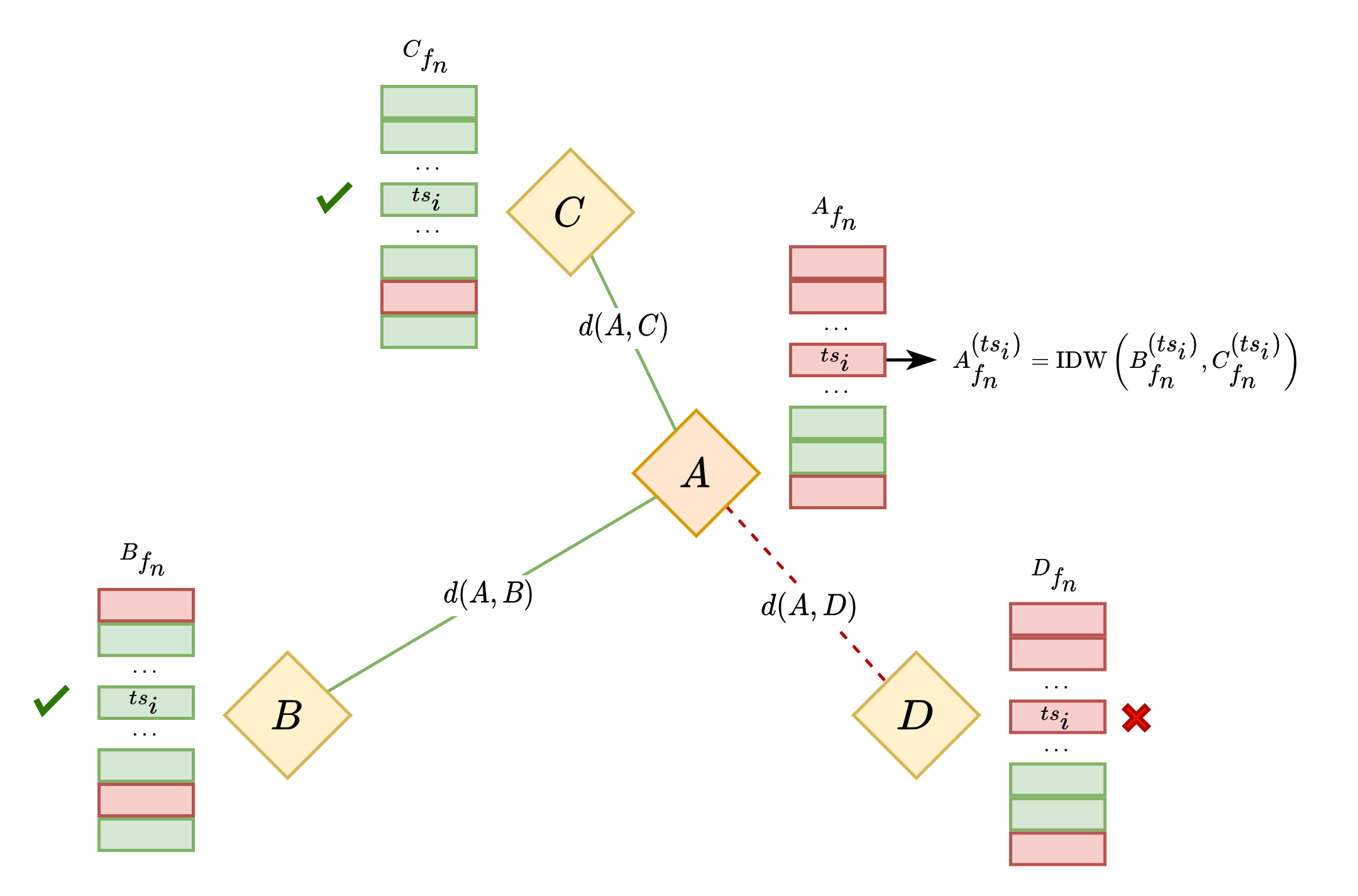
Given the amount of information lost in missing values, an imputation technique was introduced attempting to artificially reconstruct at least part of the missing data and improve training. As these phenomena are highly dependent on the geographical relation between data colecting points, specially the distance between the stations, the choice was to employ the Inverse Distance Weighting (IDW) for each of the features. The idea behind this is that closer reference values should have a greater influence in the interpolated value that reference points further apart.
The following pseudo-algorithm explains how the IDW imputation was carried out. When a station s0 is undergoing IDW imputation we first select a set of nearby_stations based on the Haversine Distance between s0 and all_avaliable_stations; then for every invalid value of feature at a timestamp t in s0, we look for valid values of feature on the same timestamp t across all selected nearby_stations. When the number valid observations in nearby_stations exceeds min_required_stations_for_imputation, feature is interpolated via IDW using the Haversine Distance as weight.
nearby_stations ← ∅

for s ∈ all_available_stations - s do
    if distance(s, s0) ⩽ maximum_imputation_distance then
        nearby_station ∪ {s}
    end
end

if |nearby_stations| ⩾ min_required_stations_for_imputation then
    for t ∈ {min(s0.timestamp), ···, max(s0.timestamp)} do
        if s0.feature at t is NULL then
            s0.feature at t ← interpolate(s0, nearby_stations, feature)
        end
    end
endFor this project this process was conducted adopting a minimum of 3 valid values to interpolate, selecting nearby stations within a maximum distance of 120km. In other words:
maximum_imputation_distance = 120min_required_stations_for_imputation = 3
The figure bellow presents a graphical representation of the same process. In this case, $A_{fn}^{(ts_i)}$ is undergoing IDW imputation using the nearby stations $B$, $C$ and $D$. As only the values in $B$ and $C$ for $f_n$ are available at $ts_i$, they will be the ones used to fill the missing $f_n$ value at $A^{(ts_i)}$. If we adopted min_required_stations_for_imputation = 3, as described below the pseudo-algorithm above, then $A_{fn}^{(ts_i)}$ would not have been imputed.
Modelling Strategy
The proposed ML-based forecasting system is composed of two stacked procedures described below. In each one of these procedures Supervised Leaning techniques have been applied in order to prepare the data and train the models.
Site-specific Models

The first step was to obtain site-specific models trained and tuned with historical meteorological data collected in each one of the collection sites of the area of study. The models and predictions in this procedure are said to be “site-specific” in the sense that, in this stage, no data is shared across stations; all training and tuning carried out in station s0 is performed only with data from s0. This is only possible bacause all stations follow the same standards when recording meteorological data. The dataset used to train the models to predict $\hat{R}_{ts + 1}$, the radiation for the next hour followed the given format:
$$ (ts, B, D, H, P, T, R, W_s, W_d) \rightarrow \hat{R}_{ts + 1} $$
The Machine Learning algorithms used to train the site-specific models are shown below. For each one of the training algorithms hyperparameters search routines also were conducted and the fitted models were all combined into a Stacking Regressor. At the end of this step we expect to produce one ensemble of trained models per meteorological station.
- Multi-layer Perceptron (Dense Neural Network - NN)
- Support Vector Machine (SVM)
- Extremely Randomized Trees (Extra Trees - ET)
- Extreme Gradient Boosting (XGB)
- Random Forests (RF)
Generalization Model

In order to generalize the predictions we need to train and tune a single generalization model using as input the predictions of the site-specific models trained in the previous procedure. For this step a new dataset is constructed from the site-specific predictions incorporating additional information. This new dataset was constructed incorporating for each station the 3-tuple $(d^n, E^n, \hat{R}_{ts_i + 1}^{n})$ in which:
- $d^n$ is the Haversine Distance from the generalized station to its $n$-th closest station.
- $E^n$ is the average between the RMSE and MAE of the estimator in the $n$-th closest station.
- $\hat{R}_{ts_i + 1}^{n}$ is the estimated value of $R$ at timestamp $ts$ produced by the $n$-th closest station.
The ideia behind it is that the generalization model should be able to learn the relations involving distance and “trustworthiness” (measured by the error $E$) of the closest nearby site-specific models when combining their predictions to produce a generalized prediction. The dataset used to train the generalization model followed the given format ($La_i$ is the latitude and $Lo_i$ of the generalized prediction site):
$$ \bigg(ts_i, La_i, Lo_i, \overbrace{d^1, E^1, \hat{R}^1}^{\text{station } 1}, \cdots, \overbrace{d^n, E^n, \hat{R}^n}^{\text{station } n} \bigg) \rightarrow {\psi_{ts + 1}} $$
To prevent noise in this new dataset, the minimum required number of tuples $(d^n, E^n, \hat{R}_{ts_i + 1}^{n})$ was set to 3. Since this dataset was set to accomomdate up to 7 of these 3-tuples, when the number of available 3-tuples was inferior to 7, the remainig “slots” were filled with zeros.
Note that:
- The filter selecting only stations with 7 years of valid retroactive observations (mentioned in section Preprocessing) was by-passed in this step as, despite not having available observations for the first procedure training, the observed values were still relevant when training and assessing the generalization model.
- When generating the dataset rows associated to a prediction site $s_i$, all predictions from this site coming from the previous stage were discarded as the distance between $s_i$ and $(La_i, Lo_i)$ is 0; so the set of selected models always considers the closest stations except the one exactly at $s_i$.
Final Prediction Scheme
Putting everything together, the following picture ilustrates the whole process of generating a solar radiation prediction. For site-specific predictions, only the inferior portion of the figure can be considered.

Baselines
As a way to assess the models and have some comparative basis two baselines were used in this project. They are described in details in the followind sections.
Empirical Model
The empirical model used in this project corresponds to the CPRG model, a decomposition-based solar radiation model capable of performing hourly predictions by relating variables such as latitude, longitude, day of year and hour with the solar radiation intensity. The implementation can be found in the project repository, for further details check out this article.
IDW-based Interpolation
This method is very similar to the Data Imputation technique used for the data imputation in the first procedure, however, instead of using IDW to interpolate values of missing features, we are interpolating predictions generated the site-specific models. As in the generalization model, this baseline model also incorporates the measure of “trustworthiness” of site-specific models by adding to the weights the error from the estimators. As a reference, the following equation shows the calculation of a weight of the model associated to a station $s_i$ with respect to the station $s_0$ ($e_{s_i}$ is the best estimator for the site $s_i$ and $d$ is the Haversine Distance).
$$ w_i(s_0,s_i) = \dfrac{1}{d(s_0, s_1)^2} \bigg( \dfrac{\text{RMSE}(e_{s_i}) + \text{MAE}(e_{s_i})}{2} \bigg)^{-1} $$
Once the weights are defined, the calculation bacomes a simple weighted sum:
$$ \psi_{ts+1} = \dfrac{\displaystyle \sum_{i=1}^k \bigg[ \overbrace{e_{s_i}(x_{s_i})}^{\hat{R}^i} \cdot w_i(s_0, s_i) \bigg]}{\displaystyle \sum_{i=1}^k w_i(s_0, s_i)} $$
Results
Given the configuration in the modelling strategy, the site-specific models and the generalization model were evaluated sepately. In both cases performance was measured using the Root Mean Squared Error (RMSE), Mean Absolute Error (MAE), the Coefficient of Determination (R²) and the Mean Bias Error (MBE). The values in the tables in upcoming sub-sections correspond to the mean ($\bar{x}$) and standard deviation of metrics values in each meteorological station comparing the results of the proposed method (ML) against its baselines.
Site-specific Models
Performance in the site-specific models was measured using the test set of each station, which corresponded data records from 2019 to 2021. The numbers presented below are the mean and standard deviantion values of the performance metrics considering the ensemble of best models obtained in each location after hyperparameter tuning.
| Metric | Method | $\underset{\text{EMP} - \text{ML}}{\Delta\%}$ | ||
|---|---|---|---|---|
| CPRG (baseline) | ML | |||
| RMSE | $\bar{x}$ | 551.68 | 363.05 | -34.19 |
| $\sigma$ | 136.97 | 43.09 | -68.53 | |
| MAE | $\bar{x}$ | 462.23 | 232.34 | -49.73 |
| $\sigma$ | 126.98 | 27.42 | -78.40 | |
| MBE | $\bar{x}$ | 184.83 | 2.25 | -98.78 |
| $\sigma$ | 36.26 | 21.31 | -41.23 | |
| R2 | $\bar{x}$ | 0.7284 | 0.8806 | 20.89 |
| $\sigma$ | 0.1370 | 0.0287 | -79.04 | |
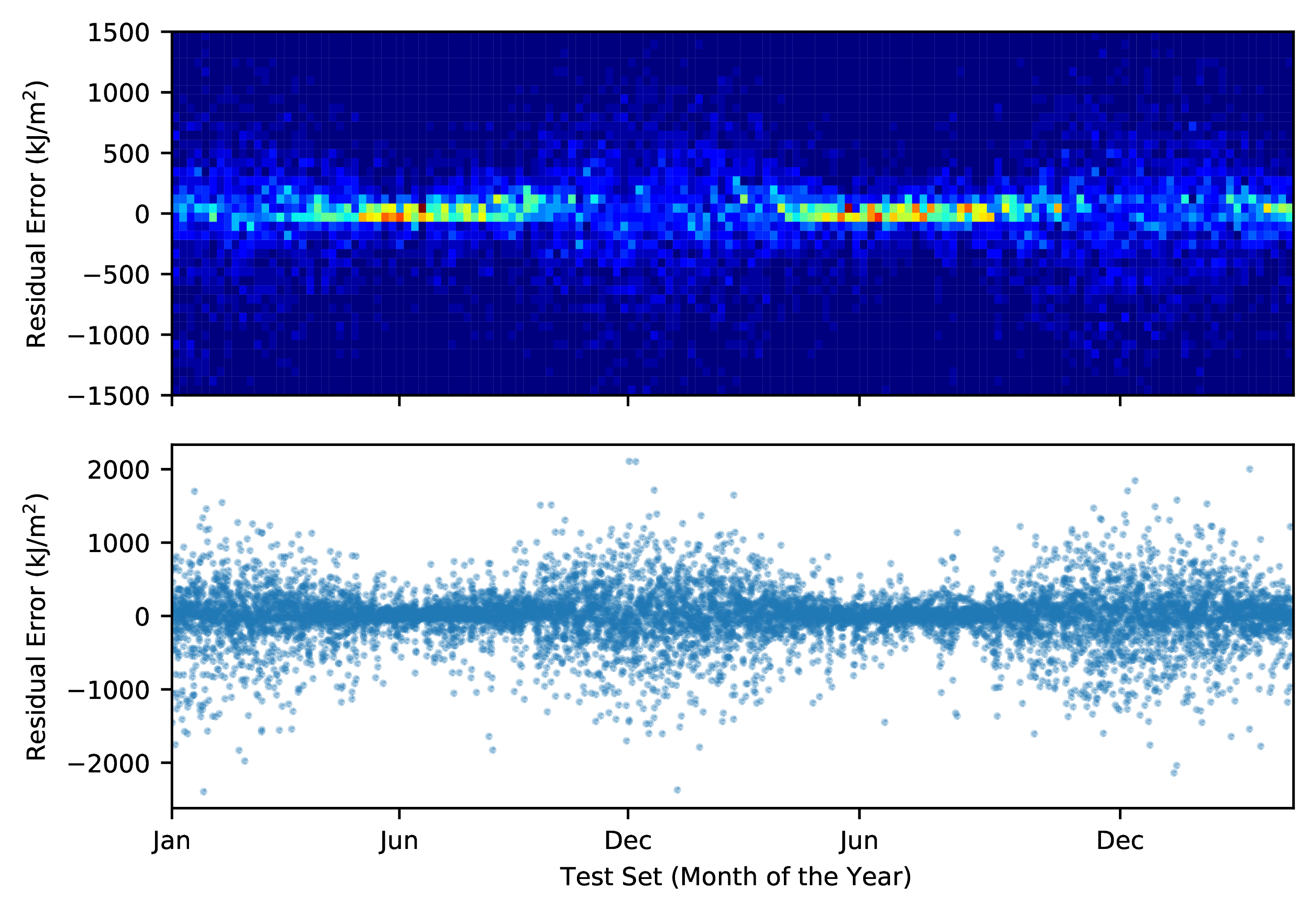
Some interesting insights were noted during the assessment in this stage. One of them was the presence of a bias in the estimators causing them to procude worse predictions along the year. This behavior, showed in the left picture below where the residual errors are plotted as a function of the day of the year in the test set, shows that higher errors are procuded in the months of November through February, which correspond to the summer rain season in this particular region. Conversely, the winters in Southeastern Brazil are characterized by the lower volume of precipitation and less variation in overall climate conditions which introduced less noise in the data consumed by the models resulting in more accurate predictions.

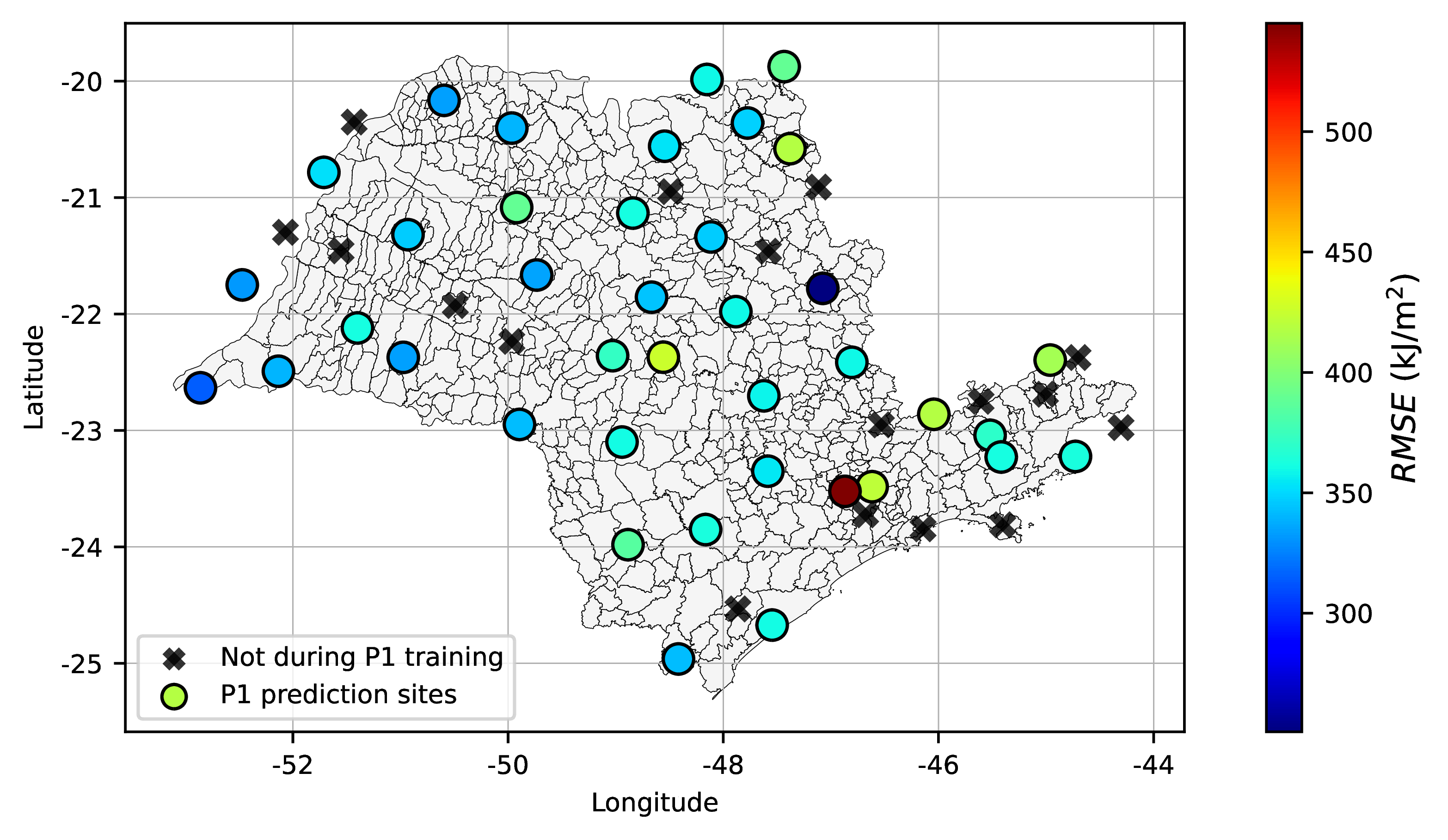
Another interesting fact was observed plotting the performance with respect to the geographical location of stations. Site-specific models located predominantly in the northwest of the State of São Paulo (see figure below) presented slightly better metrics then the ones in the Southeast. Again, this is due to the variability in climate conditions, this time influenced by the proximity of such locations to the Atlantic Ocean. Continentality of these locations make climate conditions less prone to abrupt variations; besides that, estimators also benefit from overall less precipitation as these regions are also mostly drier than other regions of the State.
Generalization Model
| Metric | Method | $\underset{\text{EMP} - \text{ML}}{\Delta\%}$ | $\underset{\text{IDW} - \text{ML}}{\Delta\%}$ | |||
|---|---|---|---|---|---|---|
| CPRG (baseline) | IDW (baseline) | ML | ||||
| RMSE | $\bar{x}$ | 535.66 | 507.73 | 392.33 | 26.74 | 22.73 |
| $\sigma$ | 128.78 | 99.86 | 58.72 | 51.38 | 41.19 | |
| MAE | $\bar{x}$ | 445.94 | 362.10 | 270.69 | 39.30 | 25.24 |
| $\sigma$ | 116.51 | 72.15 | 28.69 | 74.51 | 58.85 | |
| MBE | $\bar{x}$ | 183.81 | 0.52 | 25.25 | 86.97 | -4755.76 |
| $\sigma$ | 36.89 | 172.55 | 29.76 | 19.32 | 82.75 | |
| R2 | $\bar{x}$ | 0.7392 | 0.7581 | 0.8625 | -16.68 | -13.77 |
| $\sigma$ | 0.1344 | 0.1262 | 0.0361 | -73.14 | -71.39 | |
Conclusion
Some interesting conclusions from this project:
Both site-specific models and the generalization model were able to outperform their baselines. The difference in performance metrics between the approaches suggests that the higher cost in terms of complexity is rewarded as more accurate predictions.
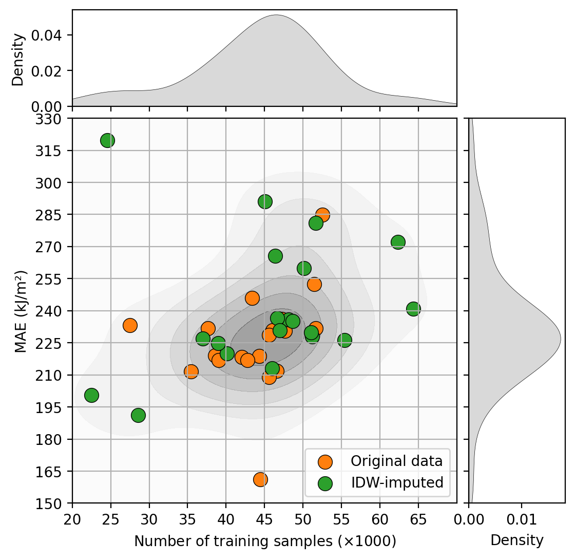
The inverse distance weighting based imputation performend during preprocessing showed to be a promising approach as an Imputation method for geographical data as more than then the half of models in P1 had their performance improved by using it. Although this technique played a relatively small role in the project, given its impact, it is fair to say that it deserves its own investigation to address further questions such as the optimal distance for imputation, how different features respond to it and its limitations and drawbacks.
The bias uncovered by residual plots may be attenuated by having models specialized in certain periods of the year. In this cases, models responsible for summertime predictions may benefit from additional techniques to reduce the excessive noise present